Cut SLO Breaches Up to 5×: LLM SLO Design for Engineers

Design LLM service-level objectives as layered targets, operational, structural, and semantic, measured at the user boundary, then enforce them with SLO-aware scheduling and layered monitoring. This combination gives inference systems a way to prioritize requests intelligently instead of treating every token the same. Recent scheduling research backs this up directly: systems built around TTFT-aware priority mapping and just-in-time bandwidth allocation report meaningfully higher SLO attainment, better goodput, and lower resource spend, with error-budget discipline from MLflow closing the observability gap.
TL;DR:
- SLOs should be layered into operational, structural, and semantic categories to effectively measure and enforce response quality and user experience.
- Prioritizing requests with SLO-aware scheduling, such as simulated annealing, can improve SLA attainment by up to five times and reduce latency by over 31 percent.
- Memory placement strategies, including disaggregation and per-request reservations, are critical for meeting latency targets during traffic spikes and long-context requests.
- Accurate measurement at the user boundary using histograms and calibrated sampling is essential for detecting and acting on actual user-perceived performance.
- Automated, continuous tuning and calibration of semantic evaluators prevent silent drift and optimize system performance across changing traffic patterns.
Table of Contents
- What Are the Three Types of SLOs for LLM Systems?
- What Components Make Up SLO-Aware Scheduling?
- How Memory Placement and Multiplexing Affect SLO Attainment
- How Do You Set Error Budgets and Alerts for LLM SLOs?
- How Do Auto-Tuning and Just-in-Time Allocation Improve SLOs?
- A Step-by-Step Recipe for Implementing LLM SLOs
- How MLflow Supports This SLO Architecture
- What I've Learned Watching These Systems Fail in Production
- Put This Playbook Into Production With MLflow
- Sources
What Are the Three Types of SLOs for LLM Systems?
Most teams default to a single latency number and call it a day. That approach breaks fast once an LLM service handles anything beyond toy traffic, because latency alone can't tell you whether the model is hallucinating, returning malformed JSON, or quietly drifting off-topic. A workable taxonomy splits SLOs into three layers, a structure recommended in recent work on designing SLOs for LLM-powered applications.
Operational SLOs cover the infrastructure basics: availability, error rate, and latency. These map cleanly onto traditional SRE practice and can be measured continuously with almost no overhead.
Structural SLOs check whether the output conforms to an expected shape, valid JSON, required fields present, no truncated responses, refusal rate within bounds. These are deterministic checks you can run on every single response without sampling.
Semantic SLOs ask whether the content is actually correct, relevant, or safe. You can't check this deterministically at scale, so it requires sampled automated evaluation calibrated against human review.
Choosing the right service-level indicators (SLIs) per layer matters as much as the taxonomy itself:
- Time to first token (TTFT) as the primary latency SLI for interactive, streaming use cases, since it tracks what users actually perceive as responsiveness.
- Inter-token latency as a diagnostic signal, not a primary SLO. It explains why TTFT or total latency drifted, but users rarely notice it directly.
- Time to total completion (TTTC) for batch or non-streaming workloads where the full response matters more than the first chunk.
- Availability and success rate as the operational floor beneath everything else.
Mapping SLIs to Critical User Journeys (CUJs), a practice borrowed from Google's SRE workbook, forces discipline here. If you can't tie an SLI to a real interaction a user cares about, it probably doesn't deserve to be an SLO. Segment queries by complexity first (short factual lookups versus long-context reasoning chains), because a single latency threshold applied uniformly across wildly different request types produces misleading attainment numbers.
Statistic to remember: Layered SLO designs that separate structural checks from semantic sampling let teams measure the majority of traffic deterministically. Semantic evaluation only needs to run on a fraction of requests with weekly calibration against human review, according to the layered SLO framework for LLM applications.
On aggregation, use percentile-based histograms (p50, p95, p99) rather than simple averages, since LLM latency distributions are heavily right-skewed by variable output lengths. A rolling 28-day window, recalibrated quarterly, gives you enough data to smooth out noisy days without hiding a slow structural regression.
What Components Make Up SLO-Aware Scheduling?
An SLO on paper does nothing until the runtime actually enforces it. That enforcement happens through a small set of coordinated components sitting between your API gateway and your model servers.
The request profiler inspects each incoming request, estimating input length, expected output length, and complexity class before the request ever reaches a GPU. The latency predictor takes that profile and forecasts how long the request will take given current queue depth and batch state. The priority mapper combines the predicted latency against the request's assigned SLO to decide where it lands in the queue, and the instance queues hold requests grouped by priority tier so the scheduler can pull from the right bucket without scanning the entire backlog.
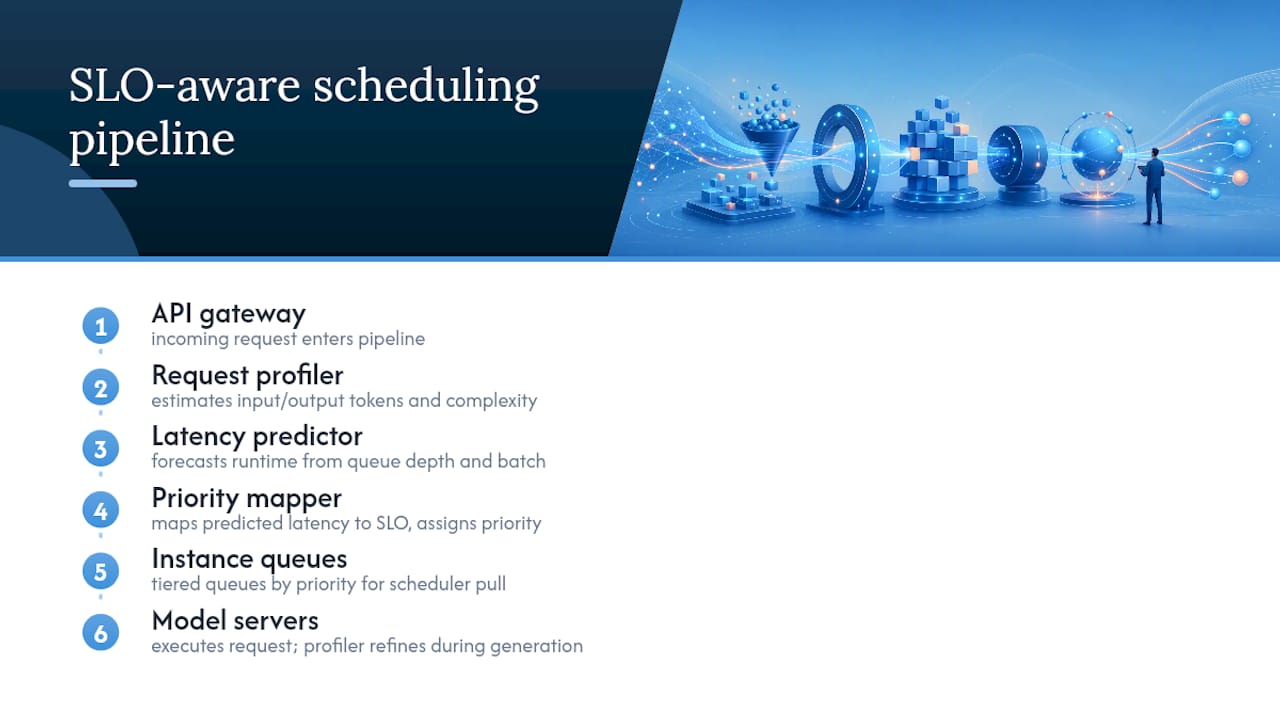
These four pieces feed each other continuously. The profiler's estimate refines as tokens actually generate, which is the core insight behind JITServe's imprecise request information approach: you don't need perfect upfront estimates if the scheduler can revise its allocation mid-generation.
Batching and priority trade-offs
Batch size is where SLO enforcement gets genuinely hard. Bigger batches improve GPU utilization and total throughput, but they also mean a fast, latency-sensitive request can get stuck behind a batch full of long-context requests. The priority mapper has to decide, request by request, whether admitting a new item into the current batch helps or hurts the SLO attainment of everything already queued.
- Heuristic priority mapping ranks requests by a weighted score combining SLO tightness, wait time, and predicted cost, then greedily assigns them to the next available batch slot.
- Simulated annealing optimization searches the space of possible batch configurations, accepting slightly worse intermediate states to escape local optima, and does it fast enough to run inline.
- Grouped just-in-time (JIT) allocation reserves bandwidth for a cluster of similar-SLO requests and refines that reservation as real token counts arrive.
- Low-overhead search trades a small amount of optimality for near-instant decisions, which matters when the scheduler itself can't become a latency bottleneck.
The empirical results here are worth taking seriously. Systems using SLO-aware priority scheduling with simulated annealing optimization report SLO attainment improvements of up to 5× and average latency reductions of up to 31.6% compared to non-SLO-aware baselines, and the optimizer itself runs with roughly 1 millisecond of overhead. That's the detail that makes this practical rather than theoretical. A scheduler that adds meaningful latency to every request in order to schedule requests well defeats its own purpose.
On the JIT allocation side, systems in the JITServe family report goodput gains of 1.4× to 6.3× and resource savings between 28.5% and 83.2%, by continuously refining bandwidth allocation as generation progresses instead of committing resources upfront based on rough estimates.
Simulated annealing and other search-based optimizers earn their complexity only once request volume and SLO tier diversity are high enough that greedy heuristics start missing attainment targets.*
How Memory Placement and Multiplexing Affect SLO Attainment
Scheduling decisions only work if the memory subsystem underneath doesn't sabotage them. This is the part of LLM SLO design most teams underestimate, because it's invisible until traffic spikes and everything queues behind a handful of long-context requests.
Colocated versus disaggregated serving is the first major fork. Colocated setups run prefill and decode on the same GPU instance, which is simpler to operate but creates head-of-line blocking: a long prefill for one request delays decode steps for every other request sharing that instance. Disaggregated serving splits prefill and decode across separate instance pools, trading operational complexity for much tighter latency isolation, particularly for TTFT.
- Rotary or rotational scheduling cycles requests through available memory slots on a fixed rhythm rather than first-come-first-served, which prevents any single long-running request from monopolizing KV cache space indefinitely.
- Memory-aware eviction policies decide which cached key-value pairs get dropped under pressure, prioritizing eviction from low-priority SLO tiers before touching high-priority requests.
- Per-request memory reservations carve out guaranteed KV cache space for high-priority tiers, so a burst of low-priority traffic can't starve latency-sensitive requests of the memory they need to keep generating.
- Prefill/decode isolation directly targets head-of-line blocking by ensuring a compute-heavy prefill phase never delays an in-progress decode phase for a different request.
Model-level architecture choices compound these runtime decisions. Comparative work on hybrid model architectures shows that block ratio choices and model slicing decisions change latency and memory footprint in ways that ripple straight through to SLO attainment. A smaller or hybrid model that fits more comfortably in available memory can hit tighter SLOs than a larger model straining against memory limits, even if the larger model wins on raw quality benchmarks.
For practical defaults, most teams do well starting with disaggregated serving once request volume justifies the added operational surface, memory reservations sized to at least cover the p95 request profile for each SLO tier, and eviction policies that never touch the top priority tier's cache under any load condition short of full outage.
How Do You Set Error Budgets and Alerts for LLM SLOs?
Everything upstream, taxonomy, scheduling, memory design, is wasted if you can't tell whether your SLOs are actually being met in production. The single most important rule here: measure at the user boundary. Internal metrics like GPU utilization or queue depth tell you about system health, but they don't tell you what a user actually experienced. A model server can report perfect internal latency while a misconfigured load balancer or retry loop doubles the latency users actually see.
Following Google's SRE guidance on implementing SLOs, the practical sequence looks like this:
- Compute SLIs from histograms captured at the API gateway or client SDK, never from internal server logs alone.
- Set SLOs with explicit target percentiles (e.g., p95 TTFT under a defined threshold) and a rolling 28-day measurement window, recalibrated quarterly as traffic patterns shift.
- Layer SLAs on top of SLOs only where contractual commitments require it. An SLA should always sit looser than the internal SLO it's built from.
- Tie every SLO to an explicit error budget: the amount of allowed failure before you halt feature rollout or scale back experimental traffic.
Statistic to remember: Google's SRE workbook recommends a fast-burn alert threshold of 14.4× the error budget consumption rate over a 1-hour window, paired with a slower window (often 6 hours or longer) to catch gradual budget drains that a fast-burn alert would miss entirely. Running both windows simultaneously avoids the two failure modes of single-window alerting: missing slow leaks or drowning in false pages from short spikes.
Tie alerts directly to enforcement. If the error budget for a semantic SLO tier drops below a defined floor, that should automatically pause rollout of new prompt versions or model updates until the team investigates, not just fire a notification into a channel nobody reads.
For telemetry beyond raw latency and error rate, sample a subset of traffic through automated semantic evaluators, run schema compliance checks on every response for structural SLOs, and make sure every SLO has a named owning team visible in your monitoring dashboard. An SLO nobody owns is an SLO nobody fixes.
How Do Auto-Tuning and Just-in-Time Allocation Improve SLOs?
Manual tuning of batch sizes, queue thresholds, and priority weights gets you through the first few months of production traffic. It stops scaling the moment you have more than two or three SLO tiers and traffic patterns that shift by time of day. Automated tuning closes that gap.
- Latency predictors fed by imprecise request signals estimate output length and complexity before generation completes, then refine those estimates as real tokens stream out, the core mechanism behind JITServe's just-in-time bandwidth allocation.
- Bayesian optimization and black-box search tune batch size, queue depth thresholds, and priority weight parameters against observed SLO attainment, without requiring an engineer to hand-derive the right values for every traffic pattern.
- Simulated annealing stays the practical favorite for inline scheduling decisions because it matches exhaustive search effectiveness while adding roughly 1 millisecond of overhead, a cost small enough to run on every scheduling decision rather than periodically.
- Calibration loops for semantic evaluators need their own tuning cycle. Sample evaluator outputs against human review regularly, because evaluator drift, where the automated judge quietly diverges from what humans would actually flag, undermines every semantic SLO built on top of it.
Pro Tip: Run your auto-tuner's proposed configuration changes through a shadow deployment before promoting them to production traffic. A tuner optimizing purely for average-case attainment can quietly sacrifice tail latency for your highest-priority tier, and you won't catch that from aggregate metrics alone.
A Step-by-Step Recipe for Implementing LLM SLOs
Here's the compact version of everything above, ordered the way you'd actually build it:
- Define Critical User Journeys before touching a single metric. If a journey doesn't exist, don't build an SLO around it.
- Choose SLIs and measurement windows per layer, TTFT for interactive latency, schema checks for structural SLOs, sampled evaluation for semantic SLOs, with a 28-day rolling window as the default.
- Instrument at the user boundary, capturing histograms at the gateway or client SDK, never relying on internal server-side timing alone.
- Implement the layered SLO model so operational, structural, and semantic targets each have distinct dashboards and owners.
- Add scheduling and memory guards, priority mapping, per-tier memory reservations, and prefill/decode isolation, to give the SLOs something enforcing them at runtime.
- Deploy sampled semantic evaluation with a defined human-review calibration cadence.
- Enforce an error-budget policy that automatically restricts rollout when budgets run low, and version your SLO definitions like code, complete with a changelog, as Google Cloud's SRE guidance recommends.
| Common mistake | Why it hurts | Fix |
|---|---|---|
| Over-aggregating latency into a single average | Hides tail latency spikes affecting your highest-value users | Use p95/p99 histograms per SLO tier |
| No named owner per SLO | Budget breaches get noticed but never fixed | Assign an owning team visible on the dashboard |
| Uncalibrated semantic evaluators | Evaluator drift silently invalidates the SLO it's meant to protect | Schedule regular human-review calibration passes |
| Treating SLA and SLO as identical | Contractual commitments end up tighter than your internal safety margin | Keep SLAs deliberately looser than internal SLOs |
How MLflow Supports This SLO Architecture
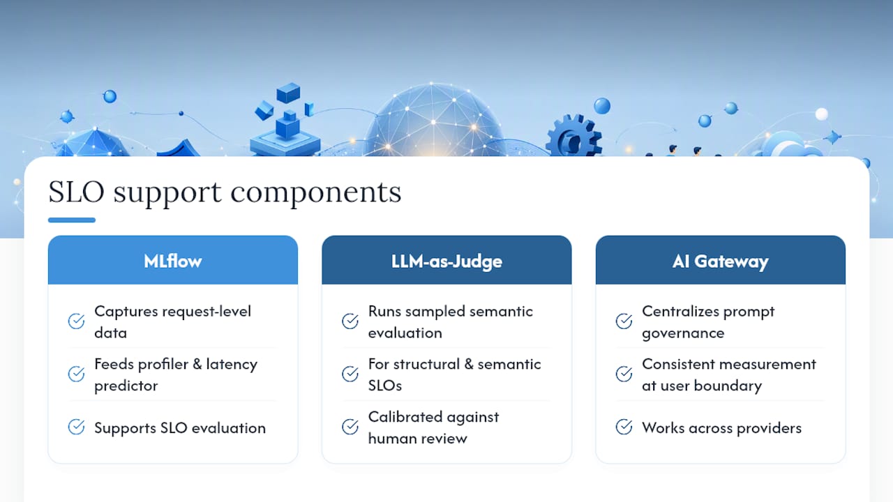
Each layer above needs a system recording and evaluating it. MLflow's tracing captures the request-level data a profiler and latency predictor depend on. LLM-as-a-Judge runs the sampled semantic evaluation your structural and semantic SLOs need, calibrated against human review. The AI Gateway centralizes prompt governance and gives you a consistent point to measure at the user boundary across providers. Teams exploring related LLM architecture patterns can see how these pieces fit a broader system design.
What I've Learned Watching These Systems Fail in Production
The failures that actually hurt teams are rarely the dramatic ones. What gets missed is the semantic SLO quietly drifting because nobody recalibrated the evaluator in three months, or the memory reservation that was sized for last quarter's traffic mix and now starves the priority tier that matters most. Layered SLOs only work if someone actually owns the middle layer, the structural checks that feel too boring to monitor and too automatable to assign a human to. Treat that ownership gap as the real risk, not the scheduling algorithm. For deeper implementation patterns, MLflow's architecture guides are worth a look.
— Kevin
Put This Playbook Into Production With MLflow
MLflow gives you the observability layer that makes every SLO tier in this playbook measurable instead of theoretical. Where most teams cobble together custom tracing scripts and ad hoc evaluation spreadsheets to check semantic correctness, MLflow's LLM-as-a-Judge evaluation runs sampled, calibrated scoring directly against your production traffic, and its tracing captures the request-level detail your latency predictor and priority mapper both need.
If you're building the request profiler, priority mapper, and error-budget enforcement described here, start by wiring MLflow's tracing into your existing gateway to get user-boundary telemetry flowing before you touch scheduling logic. Visit the Agent & LLM Engineering platform to see how orchestration, evaluation, and observability connect, or explore the documentation to scope an enterprise support engagement if your team needs hands-on integration help.
Sources
- JITServe: SLO-aware LLM Serving with Imprecise Request Information
- SLO-Aware Scheduling for Large Language Model Inferences
- SRE workbook: implementing SLOs (Google SRE guidance)