2 posts tagged with "LLM usage analytics"

LLM request tracing is the practice of recording a structured, queryable record of every call your application makes to a model, including prompts, tokens, latency, tool calls, and metadata, organized into traces and spans. It's how you debug a bad response, attribute cost to a feature, and catch quality regressions before customers do. The single most important thing to do first: instrument one endpoint with a wrapper or an OTLP exporter and confirm traces are landing somewhere you can query them.

TL;DR:

• Instrumenting a single high-traffic endpoint with SDK wrappers or OTLP is enough to start capturing useful traces before expanding to full coverage.
• Choosing a trace schema with core fields like request ID, prompt, model, token counts, and latency ensures meaningful data collection and easier troubleshooting.
• Sampling policies and PII redaction are essential to control storage costs and protect sensitive information in large-scale tracing.
• Linking evaluation scores directly to traces enables automatic detection of regressions and quality issues tied to specific prompts and model versions.
• Using MLflow's integrated observability tools simplifies setup, consolidates tracing with evaluation, and accelerates getting actionable insights in production environments.

Table of Contents​

• What an LLM Trace Actually Records (and Why It Beats Plaintext Logs)
• Choosing How to Capture Traces: SDK Wrappers, OTLP, or HTTP Interception
• A Five-Step Playbook to Start Tracing This Week
• What Traces Actually Solve Once They're Running
• Sampling, PII, and the Performance Cost Nobody Mentions
• Why Trace-Linked Evaluation Changes the Debugging Equation
• Getting Started With MLflow's Tracing and Evaluation Tools

What an LLM Trace Actually Records (and Why It Beats Plaintext Logs)​

A trace represents one full request lifecycle, from the moment a user's input hits your application to the moment a response returns. Inside that trace, each discrete operation, a model call, a retrieval lookup, a tool invocation, gets its own span. Each span can carry one or more observations: the raw inputs, outputs, and scores tied to that specific step. When an agent runs across multiple turns, a session ID ties the individual traces together so you can reconstruct the whole conversation, not just one exchange, according to the llmflow project's documentation on session correlation.

The fields worth capturing on every span:

• Request ID and timestamp, for correlation and ordering
• Full prompt (system, user, and any injected context)
• Model name and parameters (temperature, max tokens, top_p)
• Token counts, split by input and output
• Latency, measured per span and for the total trace
• Finish reason (stop, length, tool call, error)
• Tool calls and retrieval hits, with their own inputs and outputs
• Status code and any error payload

Plaintext logs bury this in unstructured strings you have to grep. A trace schema lets you filter by model, sort by latency percentile, or pull every request where token count exceeded a threshold, in a single query instead of a text search across log files.

Choosing How to Capture Traces: SDK Wrappers, OTLP, or HTTP Interception​

Three instrumentation paths dominate, and each fits a different stage of maturity. SDK wrappers hook directly into the provider client library (OpenAI, Anthropic, and similar), automatically capturing token counts and parameters with almost no code change. This is the fastest way to get useful data, but it only works where a wrapper exists for that provider.

HTTP interception sits at the network layer instead, capturing any outbound request regardless of provider or SDK version. It is more universal but requires you to parse response bodies yourself, since it has no awareness of the model's internal parameter names.

OpenTelemetry (OTLP) is the vendor-neutral option. You emit spans in the OTel format and forward them to any collector or backend that speaks the protocol. This is the path to pick if you already run an APM stack, since OpenTelemetry's specification lets LLM spans sit alongside your existing service traces rather than living in a separate silo.

Storage choice depends on scale. A single SQLite file is enough for local development or a small production service, and some lightweight open-source tracers ship with exactly that as the default, letting you migrate to ClickHouse or a managed backend once volume justifies it. Whatever you choose, make sure your session correlation attribute (a session.id or conversation.id field) is consistent across every span in a multi-turn agent, or your trace tree will fragment into disconnected fragments.

Pro Tip: Start with the SDK wrapper for your primary model provider even if you plan to move to OTLP later. You get usable traces in an afternoon instead of a sprint, and you can layer OTLP export on top once the schema is stable.

A Five-Step Playbook to Start Tracing This Week​

You don't need a platform team to get meaningful traces flowing. Here's the order that gets you from zero to production-safe fastest.

1. Pick a minimal schema. Before writing code, decide on the fields every trace must carry: request ID, timestamp, prompt, model, token counts, latency, status, and a metadata blob for anything custom. Resist the urge to capture everything on day one; a schema with eight fields you actually query beats one with thirty you don't.

2. Instrument one endpoint. Wrap a single high-traffic call, or one agent run, with your chosen method (SDK wrapper or OTLP exporter), and verify traces show up in your storage layer before touching anything else. Projects like path_tracker show a useful pattern here: log the provider, model, and full prompt/response pair alongside token counts so cost and path queries work from day one.

3. Add cost fields and evaluation hooks. Once traces are flowing, attach a computed cost field (token counts times your provider's per-token rate) and connect an automated evaluation, an LLM-as-a-Judge score, for example, to each trace. This is where regression detection starts working automatically instead of waiting for a support ticket.

4. Harden before rollout. Add sampling (trace 10 to 20% of low-value traffic, 100% of errors), PII redaction on prompt fields, asynchronous writes so tracing never blocks the response path, and a circuit breaker that disables tracing entirely if your storage backend starts timing out.

5. Build dashboards and alerts. Track p50/p95 latency, daily cost, and evaluation score trends. Alert on sudden spikes in any of the three, since a cost spike and a latency spike often share the same root cause: a prompt change that ballooned token usage.

Pro Tip: Wire your circuit breaker to fail open, not closed. If your tracing backend goes down, the LLM request should still succeed; you just lose that one trace. Losing traces is annoying. Losing production traffic because your observability layer fell over is a much worse Tuesday.

What Traces Actually Solve Once They're Running​

Traces earn their keep the first time a user reports a bad response and you can pull the exact trace tree instead of asking them to reproduce it. You see the full prompt, the model's response, and every intermediate tool call in one view, which turns a support escalation into a five-minute fix.

Beyond debugging, traces unlock a handful of concrete workflows:

• Cost attribution: token counts per trace, rolled up by feature or customer, tell you which prompts are expensive and which are just noisy.
• Agent troubleshooting: multi-step agents fail in the branch you didn't expect; a trace shows exactly which tool call or retrieval step went sideways.
• Regression detection: linking an evaluation score to every trace means a prompt change that quietly degrades quality shows up as a dip in a dashboard, not a spike in complaints.
• Usage analytics: aggregate trace data across a week or a release cycle reveals which model, provider, or prompt version is actually performing best in production, not just in your test set.

Sampling, PII, and the Performance Cost Nobody Mentions​

Tracing every request in a high-volume system gets expensive fast, both in storage and in the compute needed to write and query it. A sampling policy, full capture on errors and low-latency traffic, reduced sampling on high-volume success paths, keeps storage costs predictable without losing the traces that matter most.

Prompts and responses routinely contain names, emails, and account details. Redact or encrypt those fields at write time rather than after the fact, and gate access to raw trace data behind the same role-based controls you'd apply to production logs.

Performance-wise, synchronous trace writes are the most common mistake. Route writes through an async queue so a slow storage backend never adds latency to the user-facing request. As inference costs continue falling, Gartner projects that request volume, and the tracing load that comes with it, will keep climbing well past 2026.

• Set retention windows by trace value (errors longer, routine success shorter)
• Redact PII fields before persistence, not after
• Write traces asynchronously; never block the model response
• Alert on sudden volume or cost spikes in the tracing pipeline itself

Gartner also forecasts that explainable AI requirements will push LLM observability investment to 50% of AI budgets by 2028, which means the sampling and retention decisions you make now will only get more scrutiny, not less.

Why Trace-Linked Evaluation Changes the Debugging Equation​

Most teams treat tracing and evaluation as separate tools, one for "what happened," the other for "was it good." That split is the reason so many regressions get caught by users instead of dashboards. MLflow's approach to LLM tracing attaches LLM-as-a-Judge scores directly to individual traces, so a quality dip shows up tied to the exact prompt, model version, and input that caused it, not as an aggregate metric you have to reverse-engineer.

This matters more once you're running multiple prompt versions or model providers at once. A centralized AI Gateway with prompt versioning gives you one place to see which version is live, roll back a bad change, and audit who touched what, instead of scattering that governance across config files and Slack threads. Teams that wire evaluation scores directly to traces report catching regressions automatically rather than through manual spot-checks, which is the whole point of building this pipeline in the first place.

— Kevin

Getting Started With MLflow's Tracing and Evaluation Tools​

Tracing, automated evaluation, and prompt governance can be provided in a single open-source platform instead of stitching together three separate tools. Its LLM tracing captures the full trace/span/observation model described above, including agent tool calls and retrieval steps, and connects each trace to an LLM-as-a-Judge evaluation so regressions surface as they happen instead of after a customer notices.

If you're currently duct-taping a logging library to a spreadsheet for cost tracking, that's the exact gap MLflow's AI observability tooling is built to close, without asking you to run a separate paid backend just to get queryable traces. The GenAI platform page walks through the quickstart for agent tracing and evaluation setup, and it's a reasonable next stop if you want to see the schema and the evaluation hooks in practice before you commit engineering time to build your own.

Recommended​

• Automatically find the bad LLM responses in your LLM Evals with Cleanlab

To instrument token usage tracking correctly, capture these fields on every LLM span: input_tokens, output_tokens, total_tokens, model_name, model_provider, and a prompt_id or prompt_version. Map each model_name to a per-token pricing rate so cost can be computed immediately at the span level and aggregated up to the trace or application level.

• Minimal per-call fields: input_tokens, output_tokens, total_tokens, model_name, model_provider, prompt_id/prompt_version
• Cost attribution: measure tokens per span, then roll up to trace and application level for chargeback and budget alerts
• Implementation verdict: use auto-instrumentation when your framework supports it; otherwise annotate spans manually and maintain a model-to-pricing-rate table

Key Takeaways​

Accurate LLM cost tracking requires per-span token fields, a normalized model-to-pricing-rate table, and prompt_id tagging from the first instrumented call.

Table of Contents​

• What token usage tracking covers and why it matters for LLM teams
• Minimum requirements and quick enablement checklist
• What fields belong in your span-level data model
• How to view and query your token and cost data
• How estimated cost is computed and where precision breaks down
• Auto-instrumentation vs manual annotation: choosing your approach
• Dashboards, tagging, and cost-allocation workflows for teams
• Common mistakes when tracking tokens and how to fix them
• Mlflow-specific enablement: SDK examples, version notes, and sample span JSON
• Phased rollout from POC to production
• Why token observability is the missing layer in most LLM deployments
• Mlflow gives you production-grade token observability from day one
• Sources

What token usage tracking covers and why it matters for LLM teams​

Token usage tracking is the practice of capturing per-call token counts, mapping them to provider pricing rates, and aggregating the results into cost and quota signals your team can act on. It operates at two levels: the individual LLM span (a single API call) and the aggregated trace or application level, where you can see total spend across a user session, a feature, or a team.

The primary benefits are concrete:

• Cost visibility: know exactly what each model call costs in USD before your monthly provider bill arrives
• Model-level optimization: compare cost per request across model versions or providers to find cheaper alternatives with acceptable quality
• Chargeback and allocation: attribute spend to a team, feature, or customer tier using tags promoted to metric dimensions
• Anomaly detection: catch runaway agent loops before they burn through budget; a stuck agent can generate thousands of tokens per minute without any visible output

Units matter more than they seem. Datadog's LLM observability cost monitoring stores estimated cost in nanodollars rather than USD to avoid floating-point precision loss at the per-call level. When you aggregate millions of calls, rounding errors in USD accumulate into real accounting gaps. Storing in nanodollars and converting at display time keeps the math clean.

Trimming context cut their monthly bill significantly. Separately, a team evaluating prompt caching found that cache reads cost a fraction of standard input tokens on several major providers — but only after they started tracking cache_read_input_tokens separately from non-cached input.

For LLM performance metrics and cost tradeoffs, linking token counts to latency and error rates on the same span gives you the full picture: not just what something costs, but whether it was worth it.

Minimum requirements and quick enablement checklist​

Before you write a single line of instrumentation code, confirm these prerequisites are in place.

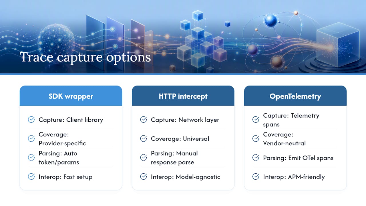
1. Choose your instrumentation path. Auto-instrumentation works out of the box for popular frameworks (OpenAI, Anthropic, LangChain, LlamaIndex) when using a supported SDK version. Manual annotation is required for custom HTTP clients, proxies, or any model not covered by an auto-instrumentation plugin.
2. Enable span token annotations. In Mlflow, set mlflow.tracing.enabled = True and confirm your SDK version supports LLM span attributes. For manual spans, call span.set_attribute("llm.token_count.prompt", n) and the equivalent completion attribute.
3. Populate model_name and model_provider on every span. These two fields are the join key between your token counts and your pricing table. Missing or inconsistent values here are the single most common cause of cost discrepancies.
4. Attach prompt_id or prompt_version. This lets you attribute cost to a specific prompt template, not just a model. Without it, you cannot tell whether a cost increase came from a model price change or a prompt that grew by 500 tokens.
5. Provide a pricing map. Maintain a YAML or JSON file that maps model_name to input_token_rate_usd and output_token_rate_usd. Update it whenever a provider changes pricing. Token Tracker surfaces a "pricing missing" badge rather than silently reporting $0 for unknown models — adopt the same pattern in your own tooling.
6. Set aggregation resolution and timezone. Decide on your rollup window (30-minute buckets for real-time dashboards, daily rollups for finance reporting) and fix the timezone to UTC to avoid billing-window mismatches across providers.
7. Define a data retention policy. Token counts and timestamps are low-risk to retain long-term. Prompt content and completions are not. Separate these from the start: store token counts in your observability backend and keep content logs, if at all, in a separate, access-controlled store.

Version note: model-name normalization is a recurring pain point. Providers return model strings like gpt-4o-2024-11-20 and gpt-4o, which are different strings but may map to the same pricing tier. Build a normalization layer that canonicalizes provider model strings before they hit your pricing table.

What fields belong in your span-level data model​

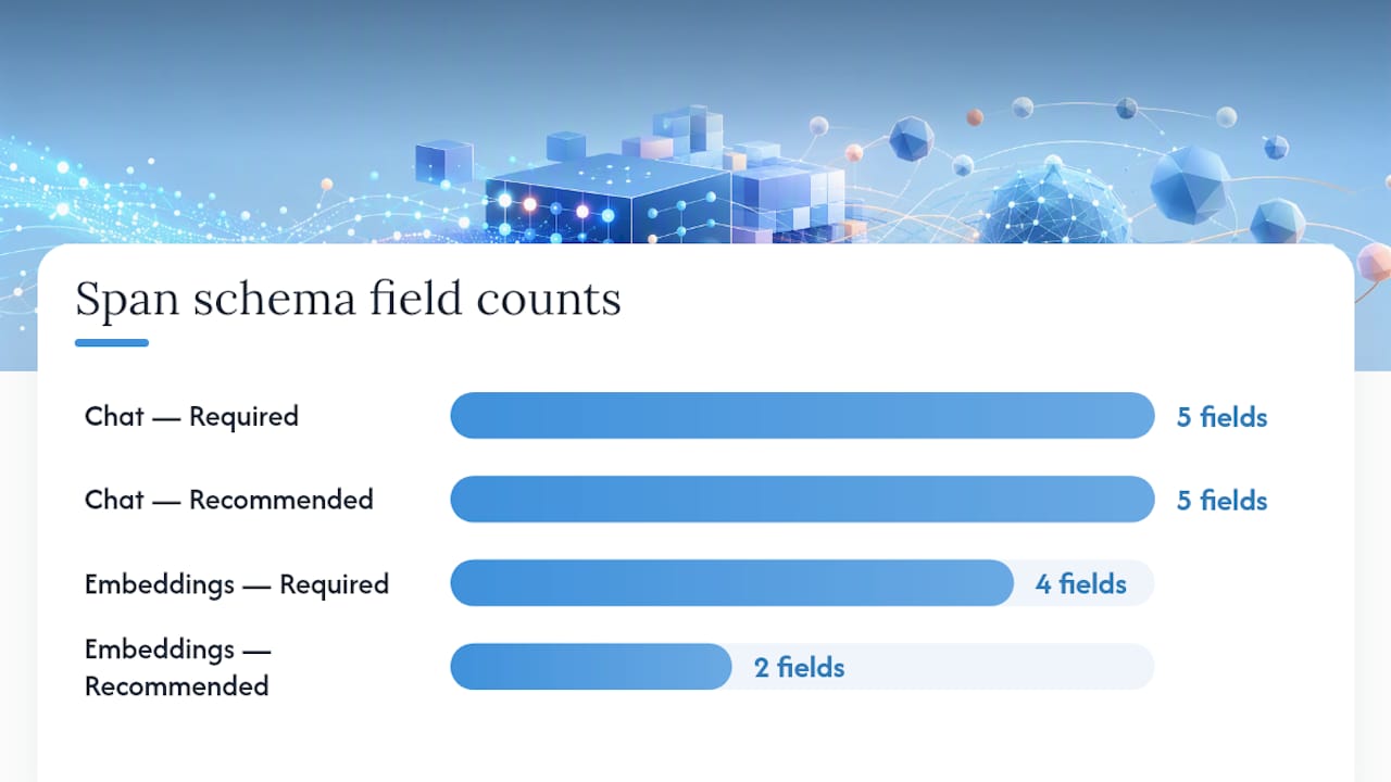
The canonical schema below is what your instrumentation should emit, whether you use auto-instrumentation or manual annotation. Getting these fields right at the span level makes every downstream aggregation and cost calculation accurate.

Parent/child relationships: when a trace contains multiple LLM spans (a multi-step agent, for example), total_tokens at the trace level is the sum of total_tokens across all child spans. Never double-count by also summing at the root span if the root span already aggregates children.

Cache token handling deserves special attention. For providers that implement prompt caching, Datadog's cost monitoring documentation notes that cache reads and cache writes carry different pricing rates than standard input tokens. If you only track input_tokens as a single field, you will overestimate cost for cache-heavy workloads and underestimate it for workloads that write large caches. The fix is straightforward: emit all three cache fields and let your pricing formula handle the rate differences.

reasoning_output_tokens matters for o-series and similar models where chain-of-thought tokens are billed separately. Omitting this field means your output cost estimate is wrong for every reasoning-model call.

How to view and query your token and cost data​

Two views serve different purposes. Per-span and per-trace views are for debugging: you open a specific trace, see which LLM call was expensive, and compare token counts against what the provider logged. Aggregated dashboards are for governance: you see total daily spend by team, cost per 1M tokens by model, and trend lines that reveal whether a new prompt version is cheaper or more expensive than the one it replaced.

Practical UI widgets to build first:

• Total cost trend (daily/weekly): a line chart of sum(estimated_cost_usd) grouped by day, filtered by environment = prod
• Cost by model: a bar chart of sum(estimated_cost_usd) grouped by model_name, useful for comparing provider costs
• Cost by prompt_id: reveals which prompt templates are the most expensive to run
• Top N expensive calls: a table of the highest-cost individual spans, sorted by estimated_cost_usd descending, with trace links for drill-down
• Cache hit impact: side-by-side of cache_read_input_tokens vs non_cached_input_tokens over time to quantify caching ROI
• Per-team cost gauge: sum(estimated_cost_usd) grouped by team tag, compared against a budget threshold

For programmatic access, LiteLLM's spend tracking API provides endpoints for daily spend breakdowns by model and provider, and per-user spend when user_id is set on each key. This pattern maps directly to a per-team or per-customer cost view: tag every request with the appropriate identifier at issuance time, then query the spend API for rollups.

Metric tags to promote from span attributes to your metrics system: team, customer_tier, feature, prompt_version, model_name, model_provider, environment. Promoting these as dimensions lets you slice any cost metric by any combination without re-querying raw spans.

How estimated cost is computed and where precision breaks down​

The formula is simple:

estimated_cost = (non_cached_input_tokens × input_rate)
               + (cache_read_input_tokens × cache_read_rate)
               + (cache_write_input_tokens × cache_write_rate)
               + (output_tokens × output_rate)
               + (reasoning_output_tokens × reasoning_rate)

Each rate is a per-token USD value from your pricing table, keyed by model_name. For a model without cache pricing, collapse the three input terms into input_tokens × input_rate.

Provider-specific price mapping is where most teams run into trouble. A model string returned by the API (claude-3-5-sonnet-20241022) must match exactly one row in your pricing table. If it does not match, you have two options: fail loudly with a "pricing missing" flag (the approach Token Tracker uses) or fall back to a parent model's rate with a warning. Silent $0 reporting is never acceptable — it makes your cost dashboards look healthy when they are not.

Why nanodollars? At $0.000003 per input token, a single call with 1,000 tokens costs $0.003. Stored as a float in USD, millions of such calls accumulate rounding errors. Stored as 3,000,000 nanodollars (integer), the math is exact. Convert to USD only at display time.

Pro Tip: When you onboard a new model, add it to your pricing table before you deploy it to production. Set a "pricing missing" alert that fires if any span's model_name has no matching pricing row. This catches new model versions that providers release mid-month without announcement.

Auto-instrumentation vs manual annotation: choosing your approach​

Auto-instrumentation is the right default when your LLM calls go through a supported client library. It captures token fields from the API response automatically, requires no changes to your application code, and stays current as provider response schemas evolve.

Manual annotation is necessary when:

• You use a custom HTTP client or an internal proxy that strips or rewrites response headers
• Your model is self-hosted and does not return standard token fields
• You need to add custom fields (prompt_id, customer_tier) that auto-instrumentation does not know about

For manual annotation in Python:

import mlflow

with mlflow.start_span(name="llm_call") as span:
    response = call_your_model(prompt)
    span.set_attribute("llm.token_count.prompt", response.usage.prompt_tokens)
    span.set_attribute("llm.token_count.completion", response.usage.completion_tokens)
    span.set_attribute("llm.token_count.total", response.usage.total_tokens)
    span.set_attribute("llm.model_name", "gpt-4o")
    span.set_attribute("llm.model_provider", "openai")
    span.set_attribute("mlflow.prompt_id", "summarize-v3")

For TypeScript:

const span = mlflow.startSpan({ name: "llm_call" });
const response = await callYourModel(prompt);
span.setAttribute("llm.token_count.prompt", response.usage.promptTokens);
span.setAttribute(
  "llm.token_count.completion",
  response.usage.completionTokens,
);
span.setAttribute("llm.model_name", "gpt-4o");
span.setAttribute("mlflow.prompt_id", "summarize-v3");
span.end();

Local-first data sources (CLI logs, JSONL files, SQLite databases) are appropriate when your team uses desktop AI coding tools that write local session logs. Tools like pitimon/TokenTracker aggregate these into 30-minute buckets and match models to a pricing snapshot without uploading any prompt content. This architecture suits multi-tool setups where each tool has its own provider billing UI.

Decision tree:

1. Does your framework have an auto-instrumentation plugin? Use it, then add custom attributes for prompt_id and team tags.
2. Are you running a proxy or gateway? Instrument at the proxy layer using the same span schema, and disable client-side instrumentation to avoid double-counting.
3. Are you parsing local CLI logs? Use a local aggregator with a pricing snapshot and export daily rollups to your central observability backend.

For AI logging best practices that apply across all three paths, the key principle is the same: separate token counts from content at the point of collection.

Dashboards, tagging, and cost-allocation workflows for teams​

Tagging is the foundation of every cost-allocation workflow. Promote these attributes as metric dimensions from the start: team, customer_tier, feature, prompt_version, model_name, model_provider, environment. Without them, you can see total spend but cannot answer "which team spent the most this week" or "did the new prompt version reduce cost."

Dashboards to build in priority order:

• Total cost trend: daily and weekly sum(estimated_cost_usd) in production, with a 7-day moving average to smooth noise
• Cost by team/feature: grouped bar chart updated daily, used for chargeback and budget reviews
• $/MTok by model: cost per million tokens for each model in use, updated as pricing tables change
• Top expensive prompts: table of prompt_id values ranked by total spend, refreshed daily
• Cache hit impact: ratio of cache_read_input_tokens to total_input_tokens over time

Alert thresholds worth configuring immediately: a sudden token-rate spike (more than 3× the 7-day average for a given model_name and team) almost always indicates a runaway agent loop. Community reports confirm that stuck agents are a leading cause of unexpected token burn in production.

For finance reconciliation, automate a daily cost export grouped by team and feature in CSV format. This gives your FinOps team a source of truth that does not require access to your observability UI. Per-customer cost views follow the same pattern: tag requests with customer_id and query sum(estimated_cost_usd) grouped by that tag.

You can also audit multiple LLMs at once to validate model-level characteristics before committing to a pricing tier, which is useful during the model-selection phase of a new feature.

Common mistakes when tracking tokens and how to fix them​

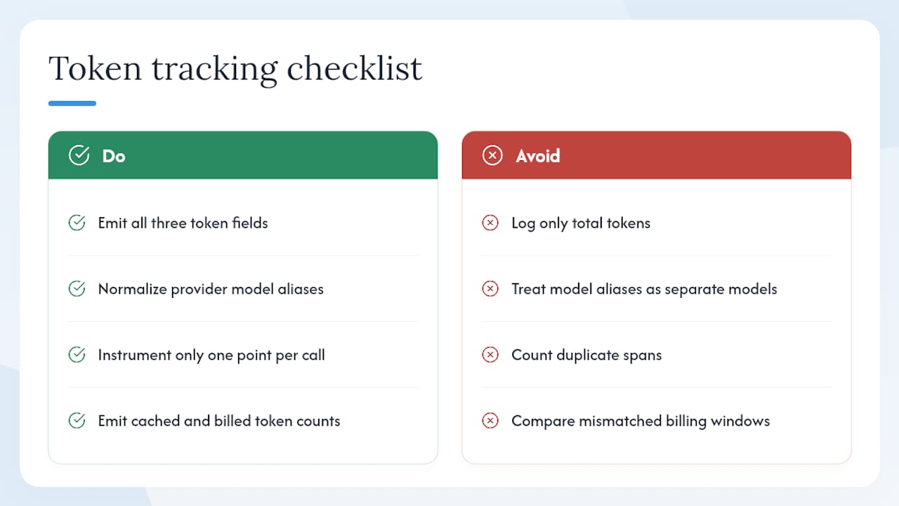
Missing token fields. The most frequent issue: a span has total_tokens but not input_tokens or output_tokens separately. This happens when teams copy a minimal logging example. Fix: always emit all three fields; infer total_tokens from the sum if the API does not return it directly.

Inconsistent model_name strings. A provider may return gpt-4o, gpt-4o-2024-11-20, or openai/gpt-4o depending on the client library version. All three are the same model but will miss your pricing table if you have only one variant. Fix: build a normalization function that maps all known aliases to a canonical key before the pricing lookup.

Double-counting when both client and proxy annotate the same call. If your application SDK and your LiteLLM proxy both emit token spans for the same request, your aggregated totals will be 2× reality. Fix: pick one instrumentation point per call path and disable the other. Use span_id deduplication in your ingestion pipeline as a safety net.

Cache misreporting. Teams that track only input_tokens without the cache breakdown overstate cost for cache-heavy workloads. The fix is to emit cache_read_input_tokens and cache_write_input_tokens separately and apply provider-specific rates to each.

Only aggregate tokens present. Some logging setups capture a session-level token total but no per-call breakdown. This makes it impossible to identify which specific call is expensive. Fix: instrument at the span level first; aggregate from there.

Debugging a cost discrepancy: align your time range to the provider's billing window (providers use different reset schedules, sometimes 5-hour UTC windows for session limits), compare your total_tokens sum against the provider dashboard for the same window, and verify that your pricing table reflects the rate that was active during that period, not the current rate.

When to re-run ingestion vs patch instrumentation: if the discrepancy is in historical data and your raw spans are intact, re-run the cost computation with a corrected pricing table. If the raw spans are missing fields, you need to patch the instrumentation and accept a gap in historical data.

Mlflow-specific enablement: SDK examples, version notes, and sample span JSON​

Mlflow's tracing system treats LLM spans as first-class citizens, capturing token fields automatically for supported integrations and providing a clean API for manual annotation.

Enable OpenAI autolog in two lines:

import mlflow
mlflow.openai.autolog()

That's it. Every subsequent OpenAI call in the process emits a span with input_tokens, output_tokens, total_tokens, model_name, and model_provider populated from the API response.

Sample span JSON (abbreviated) showing cost fields stored in nanodollars:

{
  "span_id": "abc123",
  "name": "openai.chat.completions",
  "attributes": {
    "llm.model_name": "gpt-4o",
    "llm.model_provider": "openai",
    "llm.token_count.prompt": 512,
    "llm.token_count.completion": 128,
    "llm.token_count.total": 640,
    "llm.token_count.cache_read": 256,
    "mlflow.prompt_id": "summarize-v3",
    "mlflow.estimated_cost_nanodollars": 2560000,
    "mlflow.environment": "prod",
    "mlflow.team": "search"
  },
  "start_time_unix_nano": 1718000000000000000,
  "duration_ms": 843
}

Pro Tip: Use Mlflow's prompt versioning to pin a prompt_id to every span. When you update a prompt template, increment the version and deploy. Your cost dashboards will immediately show cost per prompt version side by side, giving you a clean before/after comparison without any manual tagging. This also creates an audit trail for governance: every dollar of spend is traceable to a specific prompt version and the engineer who published it.

For AI model tracking software patterns that tie model versions to cost and correctness, Mlflow's model registry integrates with the same tracing backend, so you can correlate a cost regression with a specific model version deployment.

Phased rollout from POC to production​

A four-phase rollout keeps the scope manageable and ensures each phase produces a usable artifact before you expand.

1. POC phase (Week 1–2). Instrument 1–2 critical endpoints only. Validate input_tokens and output_tokens against your provider's usage dashboard for the same time window. Compute cost per request manually and confirm it matches your formula. Deliverable: a baseline cost-per-request figure for each instrumented endpoint.

2. Scale phase (Week 3–4). Promote team, feature, and prompt_version as metric tags. Build the total cost trend and cost-by-team dashboards. Enable the token-rate spike alert. Add per-team budget thresholds. Deliverable: a live dashboard and at least one alert firing in staging.

3. Governance phase (Week 5–6). Automate daily cost exports to your finance system. Set a data retention policy (token counts: 90 days minimum; content logs: per your data governance policy). Run a pricing-table audit: compare your stored rates against current provider pricing pages and update any stale rows. Deliverable: a recurring weekly cost review meeting with a shared dashboard link.

4. Optimization phase (ongoing). Use per-prompt_id cost data to identify candidates for prompt compression or model downgrade. Evaluate cache hit rates and adjust context-window strategies. LLM Cost Tracker tracks avoidable_cost_usd and potential_model_downgrade_savings_usd as explicit metrics — adopting similar fields in your own schema makes optimization opportunities visible without manual analysis.

Responsibilities: engineers own instrumentation and pricing-table maintenance; SRE/FinOps owns alert thresholds and budget enforcement; product owners review the weekly cost report and approve prompt changes that increase spend above a defined threshold.

Why token observability is the missing layer in most LLM deployments​

The teams that get into trouble with LLM costs are almost never the ones that ignored observability entirely. They are the ones that tracked tokens at the session or daily level but skipped the per-call span. That one gap means they can see that Tuesday was expensive but cannot tell which call, which prompt version, or which agent step caused it.

The other pattern we see repeatedly: teams that instrument tokens but never attach a prompt_id. Prompt versioning is not a nice-to-have for governance teams. It is the mechanism that makes cost changes legible to the engineers who caused them.

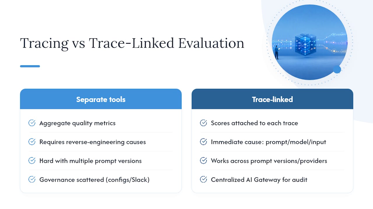
Mlflow's approach to this is to make prompt versioning and span-level tracing part of the same workflow, not two separate tools. When cost, latency, and prompt version live on the same span, the question "did this prompt change make things better or worse, and at what cost?" becomes a single query rather than a cross-system investigation.

Mlflow gives you production-grade token observability from day one​

Most teams piece together token tracking from three or four separate tools: a proxy for spend aggregation, a logging library for span data, a spreadsheet for pricing rates, and a dashboard tool for visualization. Mlflow consolidates all of that into one open-source platform with no vendor lock-in.

With Mlflow's GenAI and LLM engineering platform, you get autolog support for OpenAI, Anthropic, LangChain, and LlamaIndex out of the box, span-level token fields captured automatically, and prompt versioning that ties every dollar of spend to a specific template version. The AI Gateway adds cross-provider governance so your team can switch models without re-instrumenting. For teams ready to move from POC to production, the production observability cookbook provides step-by-step recipes for cost dashboards, alerting, and per-team budget enforcement. Start with mlflow.openai.autolog() and have your first cost dashboard running before end of day.

Sources​

• Datadog — LLM observability cost monitoring
• LiteLLM — spend tracking docs
• Token Tracker — AI token usage & cost tracker (project site)

Recommended​

• MLflow
• LLM Tracing & AI Tracing for Agents | MLflow AI Platform
• One post tagged with "monitoring LLM performance" | MLflow
• One post tagged with "best practices for LLM versioning" | MLflow