Quickstart: Compare runs, choose a model, and deploy it to a REST API

In this quickstart, you will:

• Run a hyperparameter sweep on a training script

• Compare the results of the runs in the MLflow UI

• Choose the best run and register it as a model

• Deploy the model to a REST API

• Build a container image suitable for deployment to a cloud platform

As an ML Engineer or MLOps professional, you can use MLflow to compare, share, and deploy the best models produced by the team. In this quickstart, you will use the MLflow Tracking UI to compare the results of a hyperparameter sweep, choose the best run, and register it as a model. Then, you will deploy the model to a REST API. Finally, you will create a Docker container image suitable for deployment to a cloud platform.

Set up

• Install MLflow. See the introductory quickstart for instructions

• Run the tracking server: mlflow server

Run a hyperparameter sweep

This example tries to optimize the RMSE metric of a Keras deep learning model on a wine quality dataset. It has two hyperparameters that it tries to optimize: learning-rate and momentum.

We will use the Hyperopt library to run a hyperparameter sweep across different values of learning-rate and momentum and record the results in MLflow.

Run the hyperparameter sweep, setting the MLFLOW_TRACKING_URI environment variable to the URI of the MLflow tracking server:

export MLFLOW_TRACKING_URI=http://localhost:5000

Import the following packages

import numpy as np
import pandas as pd
from hyperopt import STATUS_OK, Trials, fmin, hp, tpe
from sklearn.metrics import mean_squared_error
from sklearn.model_selection import train_test_split
from tensorflow.keras.layers import Dense, Lambda
from tensorflow.keras.models import Sequential
from tensorflow.keras.optimizers import SGD

import mlflow
from mlflow.models import infer_signature

Now load the dataset and split it into training, validation, and test sets.

# Load dataset
data = pd.read_csv(
    "https://raw.githubusercontent.com/mlflow/mlflow/master/tests/datasets/winequality-white.csv",
    sep=";",
)

# Split the data into training, validation, and test sets
train, test = train_test_split(data, test_size=0.25, random_state=42)
train_x = train.drop(["quality"], axis=1).values
train_y = train[["quality"]].values.ravel()
test_x = test.drop(["quality"], axis=1).values
test_y = test[["quality"]].values.ravel()
train_x, valid_x, train_y, valid_y = train_test_split(
    train_x, train_y, test_size=0.2, random_state=42
)
signature = infer_signature(train_x, train_y)

Then, define the model architecture and train the model. The train_model function uses MLflow to track the parameters, results, and model itself of each trial as a child run.

def train_model(params, train_x, train_y, valid_x, valid_y, test_x, test_y, epochs):
    # Define model architecture
    model = Sequential()
    model.add(
        Lambda(lambda x: (x - np.mean(train_x, axis=0)) / np.std(train_x, axis=0))
    )
    model.add(Dense(64, activation="relu", input_shape=(train_x.shape[1],)))
    model.add(Dense(1))

    # Compile model
    model.compile(
        optimizer=SGD(lr=params["lr"], momentum=params["momentum"]),
        loss="mean_squared_error",
    )

    # Train model with MLflow tracking
    with mlflow.start_run(nested=True):
        # Fit model
        model.fit(
            train_x,
            train_y,
            validation_data=(valid_x, valid_y),
            epochs=epochs,
            verbose=0,
        )

        # Evaluate the model
        predicted_qualities = model.predict(test_x)
        rmse = np.sqrt(mean_squared_error(test_y, predicted_qualities))

        # Log parameters and results
        mlflow.log_params(params)
        mlflow.log_metric("rmse", rmse)

        # Log model
        mlflow.tensorflow.log_model(model, "model", signature=signature)

        return {"loss": rmse, "status": STATUS_OK, "model": model}

The objective function takes in the hyperparameters and returns the results of the train_model function for that set of hyperparameters.

def objective(params):
    # MLflow will track the parameters and results for each run
    result = train_model(
        params,
        train_x=train_x,
        train_y=train_y,
        valid_x=valid_x,
        valid_y=valid_y,
        test_x=test_x,
        test_y=test_y,
        epochs=32,  # Or any other number of epochs
    )
    return result

Next, we will define the search space for Hyperopt. In this case, we want to try different values of learning-rate and momentum.

space = {
    "lr": hp.loguniform("lr", np.log(1e-5), np.log(1e-1)),
    "momentum": hp.uniform("momentum", 0.0, 1.0),
}

Finally, we will run the hyperparameter sweep using Hyperopt, passing in the objective function and search space. Hyperopt will try different hyperparameter combinations and return the results of the best one. We will store the best parameters, model, and rmse in MLflow.

with mlflow.start_run():
    # Conduct the hyperparameter search using Hyperopt
    trials = Trials()
    best = fmin(
        fn=objective,
        space=space,
        algo=tpe.suggest,
        max_evals=12,  # Set to a higher number to explore more hyperparameter configurations
        trials=trials,
    )

    # Fetch the details of the best run
    best_run = sorted(trials.results, key=lambda x: x["loss"])[0]

    # Log the best parameters, loss, and model
    mlflow.log_params(best)
    mlflow.log_metric("rmse", best_run["loss"])
    mlflow.tensorflow.log_model(best["model"], "model", signature=signature)

    # Print out the best parameters and corresponding loss
    print(f"Best parameters: {best}")
    print(f"Best rmse: {best_run['loss']}")

Compare the results

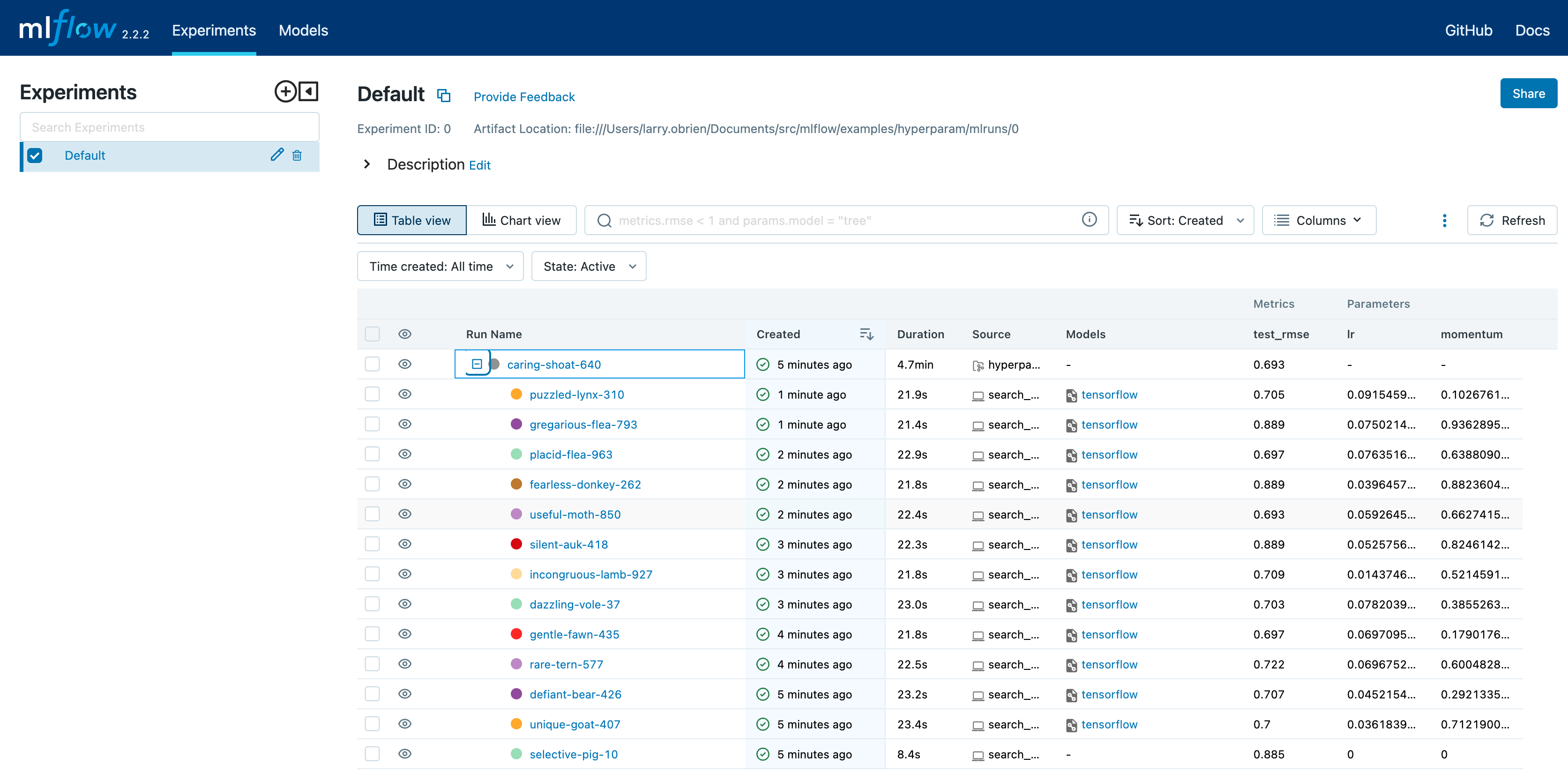
Open the MLflow UI in your browser at the MLFLOW_TRACKING_URI. You should see a nested list of runs. In the default Table view, choose the Columns button and add the Metrics | test_rmse column and the Parameters | lr and Parameters | momentum column. To sort by RMSE ascending, click the test_rmse column header. The best run typically has an RMSE on the test dataset of ~0.70. You can see the parameters of the best run in the Parameters column.

Choose Chart view. Choose the Parallel coordinates graph and configure it to show the lr and momentum coordinates and the test_rmse metric. Each line in this graph represents a run and associates each hyperparameter evaluation run’s parameters to the evaluated error metric for the run.

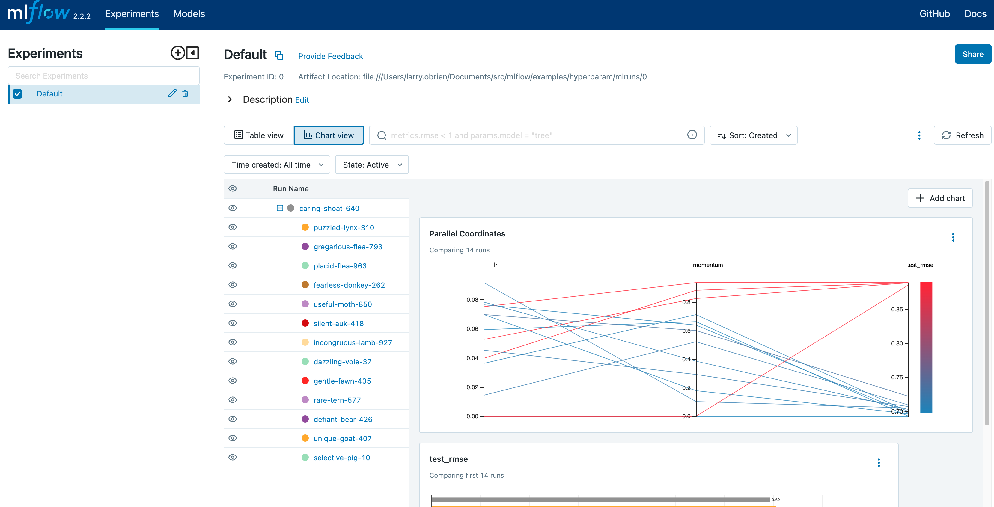
The red graphs on this graph are runs that fared poorly. The lowest one is a baseline run with both lr and momentum set to 0.0. That baseline run has an RMSE of ~0.89. The other red lines show that high momentum can also lead to poor results with this problem and architecture.

The graphs shading towards blue are runs that fared better. Hover your mouse over individual runs to see their details.

Register your best model

Choose the best run and register it as a model. In the Table view, choose the best run. In the Run Detail page, open the Artifacts section and select the Register Model button. In the Register Model dialog, enter a name for the model, such as wine-quality, and click Register.

Now, your model is available for deployment. You can see it in the Models page of the MLflow UI. Open the page for the model you just registered.

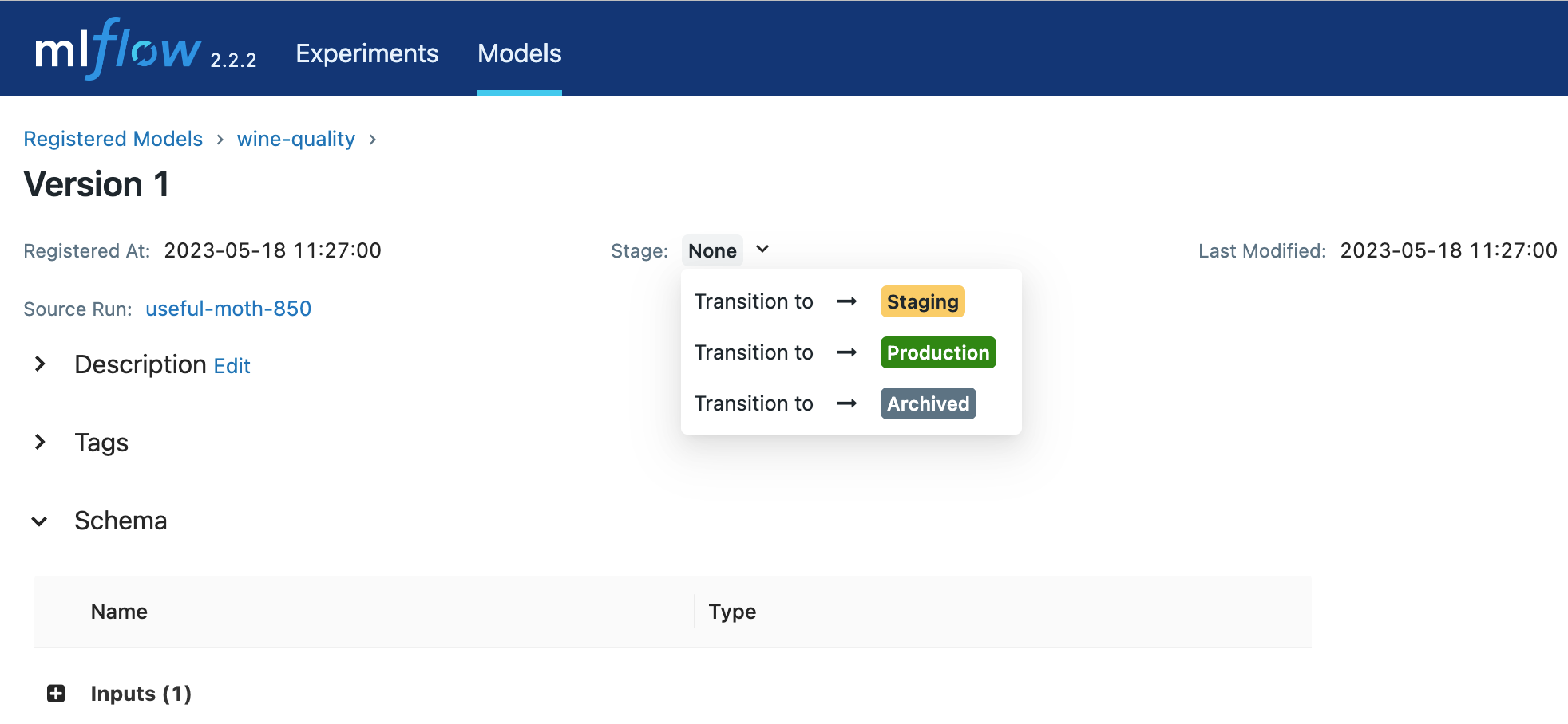
You can add a description for the model, add tags, and easily navigate back to the source run that generated this model. You can also transition the model to different stages. For example, you can transition the model to Staging to indicate that it is ready for testing. You can transition it to Production to indicate that it is ready for deployment.

Transition the model to Staging by choosing the Stage dropdown:

Serve the model locally

MLflow allows you to easily serve models produced by any run or model version. You can serve the model you just registered by running:

mlflow models serve -m "models:/wine-quality/Staging" --port 5002

(Note that specifying the port as above will be necessary if you are running the tracking server on the same machine at the default port of 5000.)

You could also have used a runs:/<run_id> URI to serve a model, or any supported URI described in Artifact Stores.

To test the model, you can send a request to the REST API using the curl command:

curl -d '{"dataframe_split": {
"columns": ["fixed acidity","volatile acidity","citric acid","residual sugar","chlorides","free sulfur dioxide","total sulfur dioxide","density","pH","sulphates","alcohol"],
"data": [[7,0.27,0.36,20.7,0.045,45,170,1.001,3,0.45,8.8]]}}' \
-H 'Content-Type: application/json' -X POST localhost:5002/invocations

Inferencing is done with a JSON POST request to the invocations path on localhost at the specified port. The columns key specifies the names of the columns in the input data. The data value is a list of lists, where each inner list is a row of data. For brevity, the above only requests one prediction of wine quality (on a scale of 3-8). The response is a JSON object with a predictions key that contains a list of predictions, one for each row of data. In this case, the response is:

{"predictions": [{"0": 5.310967445373535}]}

The schema for input and output is available in the MLflow UI in the Artifacts | Model description. The schema is available because the train.py script used the mlflow.infer_signature method and passed the result to the mlflow.log_model method. Passing the signature to the log_model method is highly recommended, as it provides clear error messages if the input request is malformed.

Build a container image for your model

Most routes toward deployment will use a container to package your model, its dependencies, and relevant portions of the runtime environment. You can use MLflow to build a Docker image for your model.

mlflow models build-docker --model-uri "models:/wine-quality/1" --name "qs_mlops"

This command builds a Docker image named qs_mlops that contains your model and its dependencies. The model-uri in this case specifies a version number (/1) rather than a lifecycle stage (/staging), but you can use whichever integrates best with your workflow. It will take several minutes to build the image. Once it completes, you can run the image to provide real-time inferencing locally, on-prem, on a bespoke Internet server, or cloud platform. You can run it locally with:

docker run -p 5002:8080 qs_mlops

This Docker run command runs the image you just built and maps port 5002 on your local machine to port 8080 in the container. You can now send requests to the model using the same curl command as before:

curl -d '{"dataframe_split": {"columns": ["fixed acidity","volatile acidity","citric acid","residual sugar","chlorides","free sulfur dioxide","total sulfur dioxide","density","pH","sulphates","alcohol"], "data": [[7,0.27,0.36,20.7,0.045,45,170,1.001,3,0.45,8.8]]}}' -H 'Content-Type: application/json' -X POST localhost:5002/invocations

Deploying to a cloud platform

Virtually all cloud platforms allow you to deploy a Docker image. The process varies considerably, so you will have to consult your cloud provider’s documentation for details.

In addition, some cloud providers have built-in support for MLflow. For instance:

• Azure ML

• Databricks

• Amazon SageMaker

• Google Cloud

all support MLflow. Cloud platforms generally support multiple workflows for deployment: command-line, SDK-based, and Web-based. You can use MLflow in any of these workflows, although the details will vary between platforms and versions. Again, you will need to consult your cloud provider’s documentation for details.