Tutorial
This tutorial showcases how you can use MLflow end-to-end to:
Train a linear regression model
Package the code that trains the model in a reusable and reproducible model format
Deploy the model into a simple HTTP server that will enable you to score predictions
This tutorial uses a dataset to predict the quality of wine based on quantitative features like the wine’s “fixed acidity”, “pH”, “residual sugar”, and so on. The dataset is from UCI’s machine learning repository. 1
Table of Contents
What You’ll Need
To run this tutorial, you’ll need to:
Install MLflow and scikit-learn. There are two options for installing these dependencies:
Install MLflow with extra dependencies, including scikit-learn (via
pip install mlflow[extras])Install MLflow (via
pip install mlflow) and install scikit-learn separately (viapip install scikit-learn)
Install conda
Clone (download) the MLflow repository via
git clone https://github.com/mlflow/mlflowcdinto theexamplesdirectory within your clone of MLflow - we’ll use this working directory for running the tutorial. We avoid running directly from our clone of MLflow as doing so would cause the tutorial to use MLflow from source, rather than your PyPI installation of MLflow.
Install conda
Install the MLflow package (via
install.packages("mlflow"))Install MLflow (via
mlflow::install_mlflow())Clone (download) the MLflow repository via
git clone https://github.com/mlflow/mlflowsetwd()into theexamplesdirectory within your clone of MLflow - we’ll use this working directory for running the tutorial. We avoid running directly from our clone of MLflow as doing so would cause the tutorial to use MLflow from source, rather than your PyPI installation of MLflow.
Training the Model
First, train a linear regression model that takes two hyperparameters: alpha and l1_ratio.
The code is located at examples/sklearn_elasticnet_wine/train.py and is reproduced below.
# The data set used in this example is from http://archive.ics.uci.edu/ml/datasets/Wine+Quality
# P. Cortez, A. Cerdeira, F. Almeida, T. Matos and J. Reis.
# Modeling wine preferences by data mining from physicochemical properties. In Decision Support Systems, Elsevier, 47(4):547-553, 2009.

import os
import warnings
import sys

import pandas as pd
import numpy as np
from sklearn.metrics import mean_squared_error, mean_absolute_error, r2_score
from sklearn.model_selection import train_test_split
from sklearn.linear_model import ElasticNet
from urllib.parse import urlparse
import mlflow
import mlflow.sklearn

import logging

logging.basicConfig(level=logging.WARN)
logger = logging.getLogger(__name__)


def eval_metrics(actual, pred):
    rmse = np.sqrt(mean_squared_error(actual, pred))
    mae = mean_absolute_error(actual, pred)
    r2 = r2_score(actual, pred)
    return rmse, mae, r2


if __name__ == "__main__":
    warnings.filterwarnings("ignore")
    np.random.seed(40)

    # Read the wine-quality csv file from the URL
    csv_url = (
        "http://archive.ics.uci.edu/ml/machine-learning-databases/wine-quality/winequality-red.csv"
    )
    try:
        data = pd.read_csv(csv_url, sep=";")
    except Exception as e:
        logger.exception(
            "Unable to download training & test CSV, check your internet connection. Error: %s", e
        )

    # Split the data into training and test sets. (0.75, 0.25) split.
    train, test = train_test_split(data)

    # The predicted column is "quality" which is a scalar from [3, 9]
    train_x = train.drop(["quality"], axis=1)
    test_x = test.drop(["quality"], axis=1)
    train_y = train[["quality"]]
    test_y = test[["quality"]]

    alpha = float(sys.argv[1]) if len(sys.argv) > 1 else 0.5
    l1_ratio = float(sys.argv[2]) if len(sys.argv) > 2 else 0.5

    with mlflow.start_run():
        lr = ElasticNet(alpha=alpha, l1_ratio=l1_ratio, random_state=42)
        lr.fit(train_x, train_y)

        predicted_qualities = lr.predict(test_x)

        (rmse, mae, r2) = eval_metrics(test_y, predicted_qualities)

        print("Elasticnet model (alpha=%f, l1_ratio=%f):" % (alpha, l1_ratio))
        print("  RMSE: %s" % rmse)
        print("  MAE: %s" % mae)
        print("  R2: %s" % r2)

        mlflow.log_param("alpha", alpha)
        mlflow.log_param("l1_ratio", l1_ratio)
        mlflow.log_metric("rmse", rmse)
        mlflow.log_metric("r2", r2)
        mlflow.log_metric("mae", mae)

        tracking_url_type_store = urlparse(mlflow.get_tracking_uri()).scheme

        # Model registry does not work with file store
        if tracking_url_type_store != "file":

            # Register the model
            # There are other ways to use the Model Registry, which depends on the use case,
            # please refer to the doc for more information:
            # https://mlflow.org/docs/latest/model-registry.html#api-workflow
            mlflow.sklearn.log_model(lr, "model", registered_model_name="ElasticnetWineModel")
        else:
            mlflow.sklearn.log_model(lr, "model")
This example uses the familiar pandas, numpy, and sklearn APIs to create a simple machine learning
model. The MLflow tracking APIs log information about each
training run, like the hyperparameters alpha and l1_ratio, used to train the model and metrics, like
the root mean square error, used to evaluate the model. The example also serializes the
model in a format that MLflow knows how to deploy.
You can run the example with default hyperparameters as follows:
# Make sure the current working directory is 'examples'
python sklearn_elasticnet_wine/train.py
Try out some other values for alpha and l1_ratio by passing them as arguments to train.py:
# Make sure the current working directory is 'examples'
python sklearn_elasticnet_wine/train.py <alpha> <l1_ratio>
Each time you run the example, MLflow logs information about your experiment runs in the directory mlruns.
Note
If you would like to use the Jupyter notebook version of train.py, try out the tutorial notebook at examples/sklearn_elasticnet_wine/train.ipynb.
The code is located at examples/r_wine/train.R and is reproduced below.
# The data set used in this example is from http://archive.ics.uci.edu/ml/datasets/Wine+Quality
# P. Cortez, A. Cerdeira, F. Almeida, T. Matos and J. Reis.
# Modeling wine preferences by data mining from physicochemical properties. In Decision Support Systems, Elsevier, 47(4):547-553, 2009.

library(mlflow)
library(glmnet)
library(carrier)

set.seed(40)

# Read the wine-quality csv file
data <- read.csv("wine-quality.csv")

# Split the data into training and test sets. (0.75, 0.25) split.
sampled <- sample(1:nrow(data), 0.75 * nrow(data))
train <- data[sampled, ]
test <- data[-sampled, ]

# The predicted column is "quality" which is a scalar from [3, 9]
train_x <- as.matrix(train[, !(names(train) == "quality")])
test_x <- as.matrix(test[, !(names(train) == "quality")])
train_y <- train[, "quality"]
test_y <- test[, "quality"]

alpha <- mlflow_param("alpha", 0.5, "numeric")
lambda <- mlflow_param("lambda", 0.5, "numeric")

with(mlflow_start_run(), {
    model <- glmnet(train_x, train_y, alpha = alpha, lambda = lambda, family= "gaussian", standardize = FALSE)
    predictor <- crate(~ glmnet::predict.glmnet(!!model, as.matrix(.x)), !!model)
    predicted <- predictor(test_x)

    rmse <- sqrt(mean((predicted - test_y) ^ 2))
    mae <- mean(abs(predicted - test_y))
    r2 <- as.numeric(cor(predicted, test_y) ^ 2)

    message("Elasticnet model (alpha=", alpha, ", lambda=", lambda, "):")
    message("  RMSE: ", rmse)
    message("  MAE: ", mae)
    message("  R2: ", r2)

    mlflow_log_param("alpha", alpha)
    mlflow_log_param("lambda", lambda)
    mlflow_log_metric("rmse", rmse)
    mlflow_log_metric("r2", r2)
    mlflow_log_metric("mae", mae)

    mlflow_log_model(predictor, "model")
})
This example uses the familiar glmnet package to create a simple machine learning
model. The MLflow tracking APIs log information about each
training run, like the hyperparameters alpha and lambda, used to train the model and metrics, like
the root mean square error, used to evaluate the model. The example also serializes the
model in a format that MLflow knows how to deploy.
You can run the example with default hyperparameters as follows:
# Make sure the current working directory is 'examples'
mlflow_run(uri = "r_wine", entry_point = "train.R")
Try out some other values for alpha and lambda by passing them as arguments to train.R:
# Make sure the current working directory is 'examples'
mlflow_run(uri = "r_wine", entry_point = "train.R", parameters = list(alpha = 0.1, lambda = 0.5))
Each time you run the example, MLflow logs information about your experiment runs in the directory mlruns.
Note
If you would like to use an R notebook version of train.R, try the tutorial notebook at examples/r_wine/train.Rmd.
Comparing the Models
Next, use the MLflow UI to compare the models that you have produced. In the same current working directory
as the one that contains the mlruns run:
mlflow ui
mlflow_ui()
and view it at http://localhost:5000.
On this page, you can see a list of experiment runs with metrics you can use to compare the models.
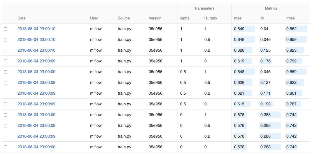
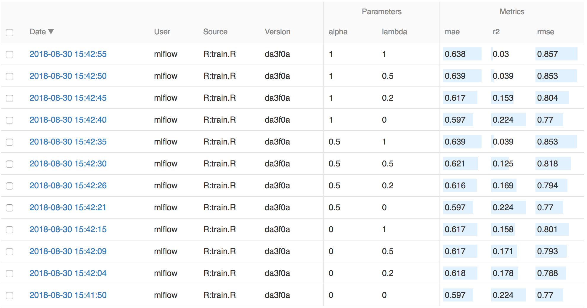
You can use the search feature to quickly filter out many models. For example, the query metrics.rmse < 0.8
returns all the models with root mean squared error less than 0.8. For more complex manipulations,
you can download this table as a CSV and use your favorite data munging software to analyze it.
Packaging Training Code in a Conda Environment
Now that you have your training code, you can package it so that other data scientists can easily reuse the model, or so that you can run the training remotely, for example on Databricks.
You do this by using MLflow Projects conventions to specify the dependencies and entry points to your code. The sklearn_elasticnet_wine/MLproject file specifies that the project has the dependencies located in a Conda environment file
called conda.yaml and has one entry point that takes two parameters: alpha and l1_ratio.
name: tutorial

conda_env: conda.yaml

entry_points:
  main:
    parameters:
      alpha: {type: float, default: 0.5}
      l1_ratio: {type: float, default: 0.1}
    command: "python train.py {alpha} {l1_ratio}"
sklearn_elasticnet_wine/conda.yaml file lists the dependencies:
name: tutorial
channels:
  - conda-forge
dependencies:
  - python=3.7
  - pip
  - pip:
      - scikit-learn==0.23.2
      - mlflow>=1.0
      - pandas
To run this project, invoke mlflow run sklearn_elasticnet_wine -P alpha=0.42. After running
this command, MLflow runs your training code in a new Conda environment with the dependencies
specified in conda.yaml.
If the repository has an MLproject file in the root you can also run a project directly from GitHub. This tutorial is duplicated in the https://github.com/mlflow/mlflow-example repository
which you can run with mlflow run https://github.com/mlflow/mlflow-example.git -P alpha=5.0.
You do this by running mlflow_snapshot() to create an R dependencies packrat file called r-dependencies.txt.
The R dependencies file lists the dependencies:
# examples/r_wine/r-dependencies.txt

PackratFormat: 1.4
PackratVersion: 0.4.9.3
RVersion: 3.5.1
Repos: CRAN=https://cran.rstudio.com/

Package: BH
Source: CRAN
Version: 1.66.0-1
Hash: 4cc8883584b955ed01f38f68bc03af6d

Package: Matrix
Source: CRAN
Version: 1.2-14
Hash: 521aa8772a1941dfdb007bf532d19dde
Requires: lattice

...
To run this project, invoke:
# Make sure the current working directory is 'examples'
mlflow_run("r_wine", entry_point = "train.R", parameters = list(alpha = 0.2))
After running this command, MLflow runs your training code in a new R session.
To restore the dependencies specified in r-dependencies.txt, you can run instead:
mlflow_restore_snapshot()
# Make sure the current working directory is 'examples'
mlflow_run("r_wine", entry_point = "train.R", parameters = list(alpha = 0.2))
You can also run a project directly from GitHub. This tutorial is duplicated in the https://github.com/rstudio/mlflow-example repository which you can run with:
mlflow_run(
  "train.R",
  "https://github.com/rstudio/mlflow-example",
  parameters = list(alpha = 0.2)
)
Specifying pip requirements using pip_requirements and extra_pip_requirements
"""
This example demonstrates how to specify pip requirements using `pip_requirements` and
`extra_pip_requirements` when logging a model via `mlflow.*.log_model`.
"""

import tempfile

import sklearn
from sklearn.datasets import load_iris
import xgboost as xgb
import mlflow
from mlflow.tracking import MlflowClient


def read_lines(path):
    with open(path) as f:
        return f.read().splitlines()


def get_pip_requirements(run_id, artifact_path, return_constraints=False):
    client = MlflowClient()
    req_path = client.download_artifacts(run_id, f"{artifact_path}/requirements.txt")
    reqs = read_lines(req_path)

    if return_constraints:
        con_path = client.download_artifacts(run_id, f"{artifact_path}/constraints.txt")
        cons = read_lines(con_path)
        return set(reqs), set(cons)

    return set(reqs)


def main():
    iris = load_iris()
    dtrain = xgb.DMatrix(iris.data, iris.target)
    model = xgb.train({}, dtrain)

    xgb_req = f"xgboost=={xgb.__version__}"
    sklearn_req = f"scikit-learn=={sklearn.__version__}"

    with mlflow.start_run() as run:
        run_id = run.info.run_id

        # Default (both `pip_requirements` and `extra_pip_requirements` are unspecified)
        artifact_path = "default"
        mlflow.xgboost.log_model(model, artifact_path)
        pip_reqs = get_pip_requirements(run_id, artifact_path)
        assert pip_reqs.issuperset(["mlflow", xgb_req]), pip_reqs

        # Overwrite the default set of pip requirements using `pip_requirements`
        artifact_path = "pip_requirements"
        mlflow.xgboost.log_model(model, artifact_path, pip_requirements=[sklearn_req])
        pip_reqs = get_pip_requirements(run_id, artifact_path)
        assert pip_reqs == {"mlflow", sklearn_req}, pip_reqs

        # Add extra pip requirements on top of the default set of pip requirements
        # using `extra_pip_requirements`
        artifact_path = "extra_pip_requirements"
        mlflow.xgboost.log_model(model, artifact_path, extra_pip_requirements=[sklearn_req])
        pip_reqs = get_pip_requirements(run_id, artifact_path)
        assert pip_reqs.issuperset(["mlflow", xgb_req, sklearn_req]), pip_reqs

        # Specify pip requirements using a requirements file
        with tempfile.NamedTemporaryFile("w", suffix=".requirements.txt") as f:
            f.write(sklearn_req)
            f.flush()

            # Path to a pip requirements file
            artifact_path = "requirements_file_path"
            mlflow.xgboost.log_model(model, artifact_path, pip_requirements=f.name)
            pip_reqs = get_pip_requirements(run_id, artifact_path)
            assert pip_reqs == {"mlflow", sklearn_req}, pip_reqs

            # List of pip requirement strings
            artifact_path = "requirements_file_list"
            mlflow.xgboost.log_model(
                model, artifact_path, pip_requirements=[xgb_req, f"-r {f.name}"]
            )
            pip_reqs = get_pip_requirements(run_id, artifact_path)
            assert pip_reqs == {"mlflow", xgb_req, sklearn_req}, pip_reqs

        # Using a constraints file
        with tempfile.NamedTemporaryFile("w", suffix=".constraints.txt") as f:
            f.write(sklearn_req)
            f.flush()

            artifact_path = "constraints_file"
            mlflow.xgboost.log_model(
                model, artifact_path, pip_requirements=[xgb_req, f"-c {f.name}"]
            )
            pip_reqs, pip_cons = get_pip_requirements(
                run_id, artifact_path, return_constraints=True
            )
            assert pip_reqs == {"mlflow", xgb_req, "-c constraints.txt"}, pip_reqs
            assert pip_cons == {sklearn_req}, pip_cons


if __name__ == "__main__":
    main()
Serving the Model
Now that you have packaged your model using the MLproject convention and have identified the best model, it is time to deploy the model using MLflow Models. An MLflow Model is a standard format for packaging machine learning models that can be used in a variety of downstream tools — for example, real-time serving through a REST API or batch inference on Apache Spark.
In the example training code, after training the linear regression model, a function in MLflow saved the model as an artifact within the run.
mlflow.sklearn.log_model(lr, "model")
To view this artifact, you can use the UI again. When you click a date in the list of experiment runs you’ll see this page.
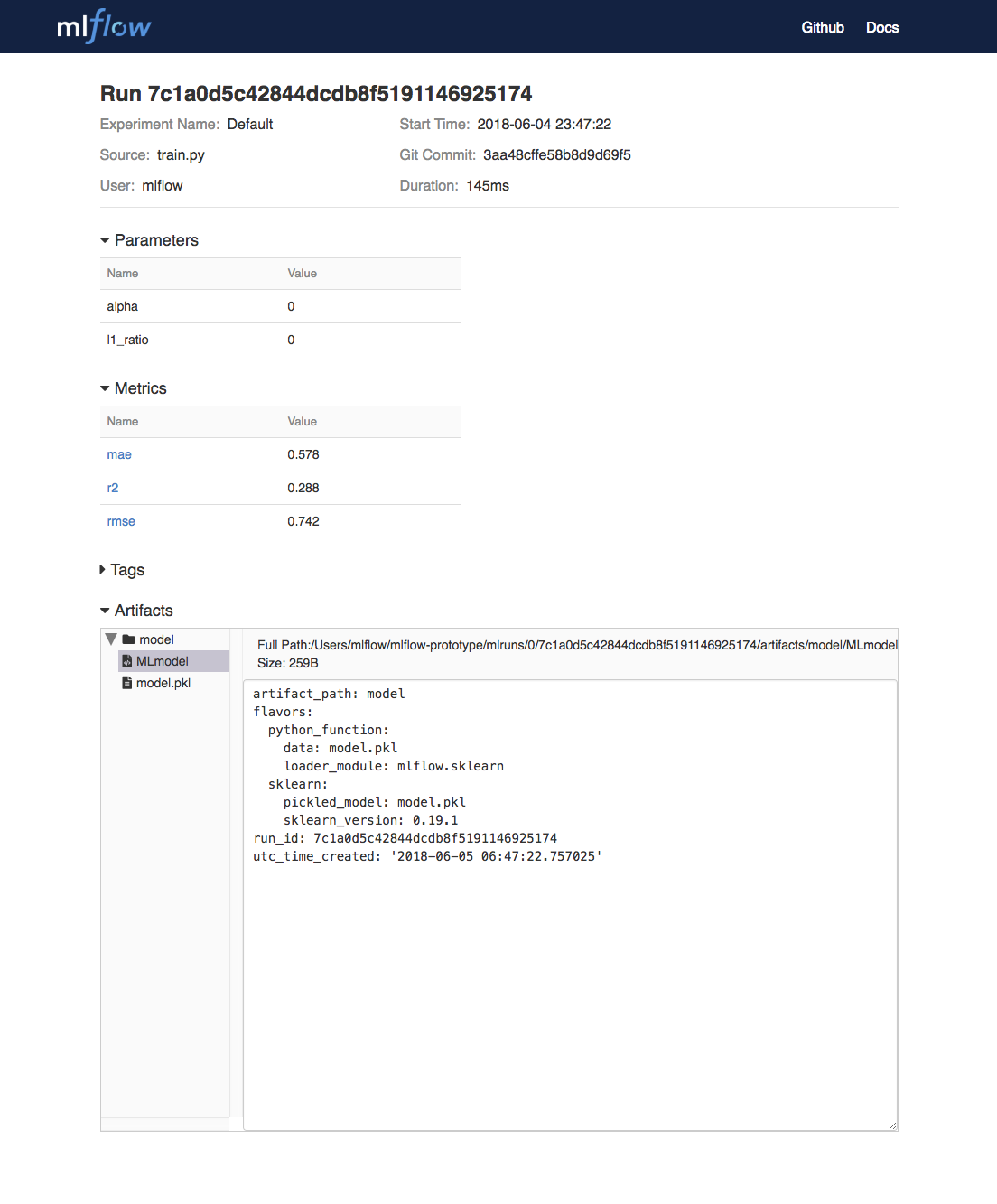
At the bottom, you can see that the call to mlflow.sklearn.log_model produced two files in
/Users/mlflow/mlflow-prototype/mlruns/0/7c1a0d5c42844dcdb8f5191146925174/artifacts/model.
The first file, MLmodel, is a metadata file that tells MLflow how to load the model. The
second file, model.pkl, is a serialized version of the linear regression model that you trained.
In this example, you can use this MLmodel format with MLflow to deploy a local REST server that can serve predictions.
To deploy the server, run (replace the path with your model’s actual path):
mlflow models serve -m /Users/mlflow/mlflow-prototype/mlruns/0/7c1a0d5c42844dcdb8f5191146925174/artifacts/model -p 1234
Note
The version of Python used to create the model must be the same as the one running mlflow models serve.
If this is not the case, you may see the error
UnicodeDecodeError: 'ascii' codec can't decode byte 0x9f in position 1: ordinal not in range(128)
or raise ValueError, "unsupported pickle protocol: %d".
Once you have deployed the server, you can pass it some sample data and see the
predictions. The following example uses curl to send a JSON-serialized pandas DataFrame
with the split orientation to the model server. For more information about the input data
formats accepted by the model server, see the
MLflow deployment tools documentation.
# On Linux and macOS
curl -X POST -H "Content-Type:application/json; format=pandas-split" --data '{"columns":["alcohol", "chlorides", "citric acid", "density", "fixed acidity", "free sulfur dioxide", "pH", "residual sugar", "sulphates", "total sulfur dioxide", "volatile acidity"],"data":[[12.8, 0.029, 0.48, 0.98, 6.2, 29, 3.33, 1.2, 0.39, 75, 0.66]]}' http://127.0.0.1:1234/invocations

# On Windows
curl -X POST -H "Content-Type:application/json; format=pandas-split" --data "{\"columns\":[\"alcohol\", \"chlorides\", \"citric acid\", \"density\", \"fixed acidity\", \"free sulfur dioxide\", \"pH\", \"residual sugar\", \"sulphates\", \"total sulfur dioxide\", \"volatile acidity\"],\"data\":[[12.8, 0.029, 0.48, 0.98, 6.2, 29, 3.33, 1.2, 0.39, 75, 0.66]]}" http://127.0.0.1:1234/invocations
the server should respond with output similar to:
[6.379428821398614]
mlflow_log_model(predictor, "model")
To view this artifact, you can use the UI again. When you click a date in the list of experiment runs you’ll see this page.
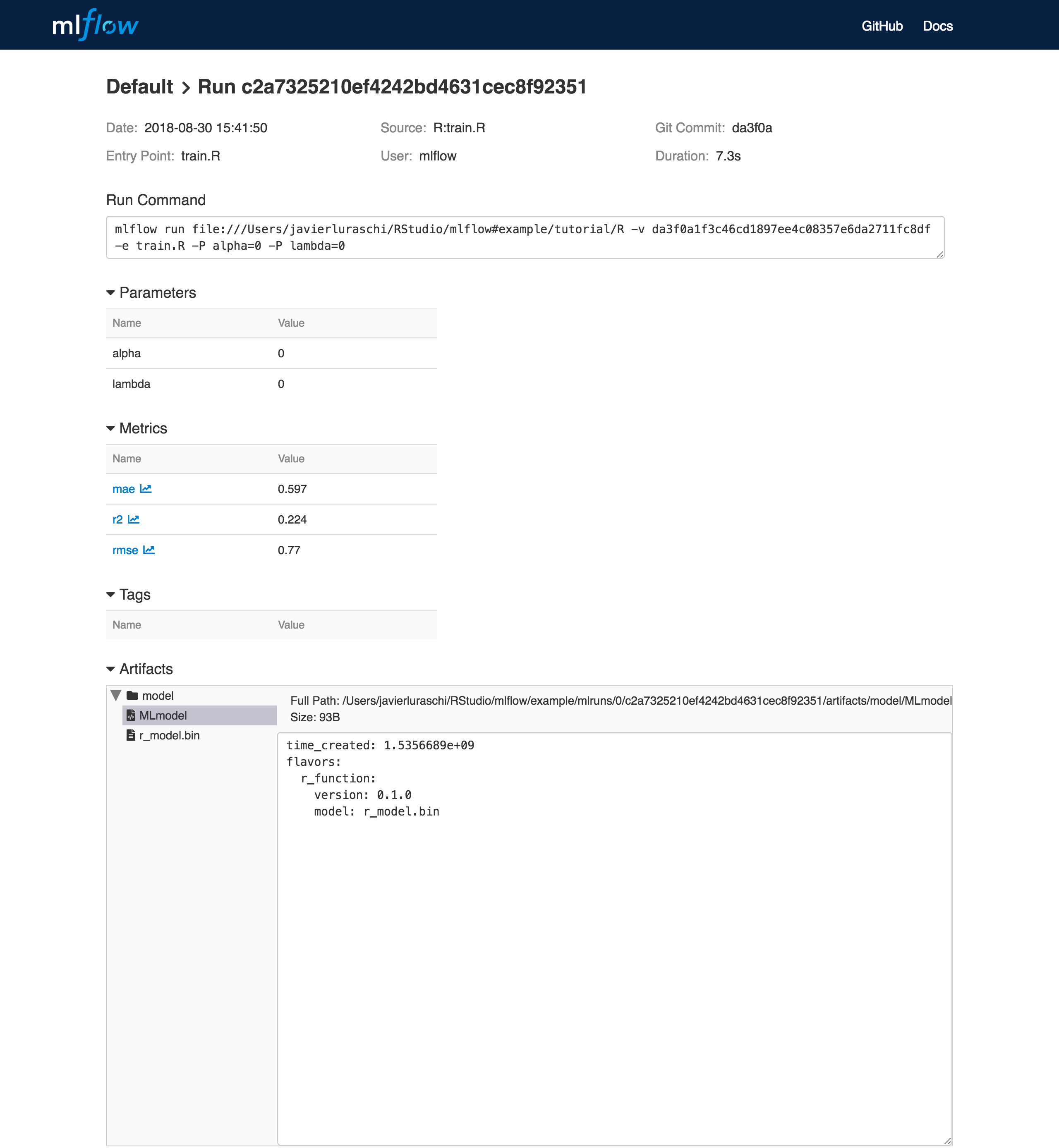
At the bottom, you can see that the call to mlflow_log_model() produced two files in
mlruns/0/c2a7325210ef4242bd4631cec8f92351/artifacts/model/.
The first file, MLmodel, is a metadata file that tells MLflow how to load the model. The
second file, r_model.bin, is a serialized version of the linear regression model that you trained.
In this example, you can use this MLmodel format with MLflow to deploy a local REST server that can serve predictions.
To deploy the server, run:
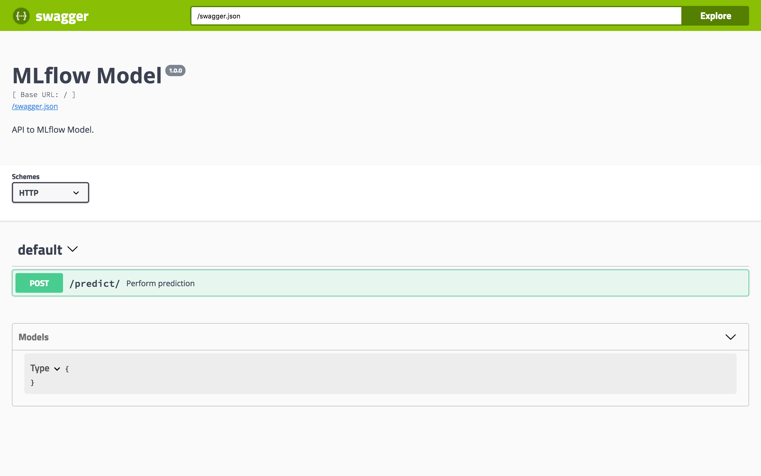
mlflow_rfunc_serve(model_uri="mlruns/0/c2a7325210ef4242bd4631cec8f92351/artifacts/model", port=8090)
This initializes a REST server and opens a Swagger interface to perform predictions against the REST API:
Note
By default, a model is served using the R packages available. To ensure the environment serving
the prediction function matches the model, set restore = TRUE when calling
mlflow_rfunc_serve().
To serve a prediction, enter this in the Swagger UI:
{
  "fixed acidity": 6.2,
  "volatile acidity": 0.66,
  "citric acid": 0.48,
  "residual sugar": 1.2,
  "chlorides": 0.029,
  "free sulfur dioxide": 29,
  "total sulfur dioxide": 75,
  "density": 0.98,
  "pH": 3.33,
  "sulphates": 0.39,
  "alcohol": 12.8
}
which should return something like:
[
  [
    6.4287492410792
  ]
]
Or run:
# On Linux and macOS
curl -X POST "http://127.0.0.1:8090/predict/" -H "accept: application/json" -H "Content-Type: application/json" -d "{"fixed acidity": 6.2, "volatile acidity": 0.66, "citric acid": 0.48, "residual sugar": 1.2, "chlorides": 0.029, "free sulfur dioxide": 29, "total sulfur dioxide": 75, "density": 0.98, "pH": 3.33, "sulphates": 0.39, "alcohol": 12.8}"

# On Windows
curl -X POST "http://127.0.0.1:8090/predict/" -H "accept: application/json" -H "Content-Type: application/json" -d "{\"fixed acidity\": 6.2, \"volatile acidity\": 0.66, \"citric acid\": 0.48, \"residual sugar\": 1.2, \"chlorides\": 0.029, \"free sulfur dioxide\": 29, \"total sulfur dioxide\": 75, \"density\": 0.98, \"pH\": 3.33, \"sulphates\": 0.39, \"alcohol\": 12.8}"
the server should respond with output similar to:
[[6.4287492410792]]
Deploy the Model to Seldon Core or KServe (experimental)
After training and testing our model, we are now ready to deploy it to production. MLflow allows you to serve your model using MLServer, which is already used as the core Python inference server in Kubernetes-native frameworks including Seldon Core and KServe (formerly known as KFServing). Therefore, we can leverage this support to build a Docker image compatible with these frameworks.
Note
Note that this an optional step, which is currently only available for Python models. Besides this, it’s also worth noting that:
This feature is experimental and is subject to change.
MLServer requires Python 3.7 or above.
This step requires some basic Kubernetes knowledge, including familiarity with
kubectl.
To build a Docker image containing our model, we can use the mlflow models
build-docker subcommand, alongside the --enable-mlserver flag.
For example, to build a image named my-docker-image, we could do:
mlflow models build-docker \
-m /Users/mlflow/mlflow-prototype/mlruns/0/7c1a0d5c42844dcdb8f5191146925174/artifacts/model \
-n my-docker-image \
--enable-mlserver
Once we have our image built, the next step will be to deploy it to our
cluster.
One way to do this is by applying the respective Kubernetes manifests through
the kubectl CLI:
kubectl apply -f my-manifest.yaml
This step assumes that you’ve got kubectl access to a Kubernetes
cluster already setup with Seldon Core.
To read more on how to set this up, you can refer to the Seldon Core
quickstart guide.
apiVersion: machinelearning.seldon.io/v1
kind: SeldonDeployment
metadata:
  name: mlflow-model
spec:
  predictors:
    - name: default
      annotations:
        seldon.io/no-engine: "true"
      graph:
        name: mlflow-model
        type: MODEL
      componentSpecs:
        - spec:
            containers:
              - name: mlflow-model
                image: my-docker-image
                imagePullPolicy: IfNotPresent
                securityContext:
                  runAsUser: 0
                ports:
                  - containerPort: 8080
                    name: http
                    protocol: TCP
                  - containerPort: 8081
                    name: grpc
                    protocol: TCP
This step assumes that you’ve got kubectl access to a Kubernetes
cluster already setup with KServe.
To read more on how to set this up, you can refer to the KServe
quickstart guide.
apiVersion: serving.kserve.io/v1beta1
kind: InferenceService
metadata:
  name: mlflow-model
spec:
  predictor:
    containers:
      - name: mlflow-model
        image: my-docker-image
        ports:
          - containerPort: 8080
            protocol: TCP
        env:
          - name: PROTOCOL
            value: v2
More Resources
Congratulations on finishing the tutorial! For more reading, see MLflow Tracking, MLflow Projects, MLflow Models, and more.
- 1
Cortez, A. Cerdeira, F. Almeida, T. Matos and J. Reis. Modeling wine preferences by data mining from physicochemical properties. In Decision Support Systems, Elsevier, 47(4):547-553, 2009.